US Investment Data

US data for fitting an investment equation.

data(Investment)

Format

An annual time series from 1963 to 1982 with 7 variables.

GNP

nominal gross national product (in billion USD),

Investment

nominal gross private domestic investment (in billion USD),

Price

price index, implicit price deflator for GNP,

Interest

interest rate, average yearly discount rate charged by the New York Federal Reserve Bank,

RealGNP

real GNP (= GNP/Price),

RealInv

real investment (= Investment/Price),

RealInt

approximation to the real interest rate (= Interest - 100 * diff(Price)/Price).

Source

Table 15.1 in Greene (1993)

References

Greene W.H. (1993). Econometric Analysis, 2nd edition. Macmillan Publishing Company, New York.

Executive Office of the President (1984). Economic Report of the President. US Government Printing Office, Washington, DC.

Examples

## Willam H. Greene, Econometric Analysis, 2nd Ed.
## Chapter 15
## load data set, p. 411, Table 15.1
data(Investment)

## fit linear model, p. 412, Table 15.2
fm <- lm(RealInv ~ RealGNP + RealInt, data = Investment)
summary(fm)
#> 
#> Call:
#> lm(formula = RealInv ~ RealGNP + RealInt, data = Investment)
#> 
#> Residuals:
#>     Min      1Q  Median      3Q     Max 
#> -34.987  -6.638   0.180  10.408  26.288 
#> 
#> Coefficients:
#>              Estimate Std. Error t value Pr(>|t|)    
#> (Intercept) -12.53360   24.91527  -0.503    0.622    
#> RealGNP       0.16914    0.02057   8.224 3.87e-07 ***
#> RealInt      -1.00144    2.36875  -0.423    0.678    
#> ---
#> Signif. codes:  0 ‘***’ 0.001 ‘**’ 0.01 ‘*’ 0.05 ‘.’ 0.1 ‘ ’ 1
#> 
#> Residual standard error: 17.21 on 16 degrees of freedom
#>   (1 observation deleted due to missingness)
#> Multiple R-squared:  0.8141,	Adjusted R-squared:  0.7908 
#> F-statistic: 35.03 on 2 and 16 DF,  p-value: 1.429e-06
#> 

## visualize residuals, p. 412, Figure 15.1
plot(ts(residuals(fm), start = 1964),
  type = "b", pch = 19, ylim = c(-35, 35), ylab = "Residuals")
sigma <- sqrt(sum(residuals(fm)^2)/fm$df.residual) ## maybe used df = 26 instead of 16 ??
abline(h = c(-2, 0, 2) * sigma, lty = 2)


if(require(lmtest)) {
## Newey-West covariances, Example 15.3
coeftest(fm, vcov = NeweyWest(fm, lag = 4))
## Note, that the following is equivalent:
coeftest(fm, vcov = kernHAC(fm, kernel = "Bartlett", bw = 5, prewhite = FALSE, adjust = FALSE))

## Durbin-Watson test, p. 424, Example 15.4
dwtest(fm)

## Breusch-Godfrey test, p. 427, Example 15.6
bgtest(fm, order = 4)
}
#> Loading required package: lmtest
#> Loading required package: zoo
#> 
#> Attaching package: ‘zoo’
#> The following objects are masked from ‘package:base’:
#> 
#>     as.Date, as.Date.numeric
#> 
#> 	Breusch-Godfrey test for serial correlation of order up to 4
#> 
#> data:  fm
#> LM test = 12.07, df = 4, p-value = 0.01684
#> 

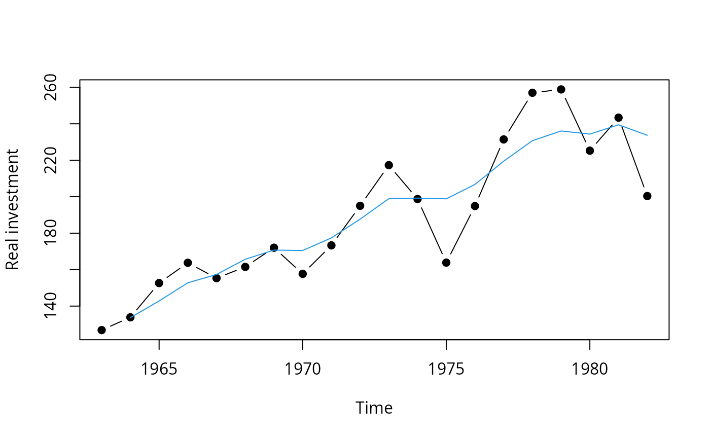
## visualize fitted series
plot(Investment[, "RealInv"], type = "b", pch = 19, ylab = "Real investment")
lines(ts(fitted(fm), start = 1964), col = 4)



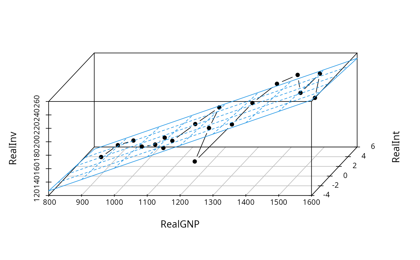
## 3-d visualization of fitted model
if(require(scatterplot3d)) {
s3d <- scatterplot3d(Investment[,c(5,7,6)],
  type = "b", angle = 65, scale.y = 1, pch = 16)
s3d$plane3d(fm, lty.box = "solid", col = 4)
}
#> Loading required package: scatterplot3d