US Expenditures for Public Schools

Per capita expenditure on public schools and per capita income by state in 1979.

data("PublicSchools")

Format

A data frame containing 51 observations of 2 variables.

Expenditure

per capita expenditure on public schools,

Income

per capita income.

Source

Table 14.1 in Greene (1993)

References

Cribari-Neto F. (2004). “Asymptotic Inference Under Heteroskedasticity of Unknown Form.” Computational Statistics & Data Analysis, 45, 215-233.

Greene W.H. (1993). Econometric Analysis, 2nd edition. Macmillan Publishing Company, New York.

US Department of Commerce (1979). Statistical Abstract of the United States. US Government Printing Office, Washington, DC.

Examples

## Willam H. Greene, Econometric Analysis, 2nd Ed.
## Chapter 14
## load data set, p. 385, Table 14.1
data("PublicSchools", package = "sandwich")

## omit NA in Wisconsin and scale income
ps <- na.omit(PublicSchools)
ps$Income <- ps$Income * 0.0001

## fit quadratic regression, p. 385, Table 14.2
fmq <- lm(Expenditure ~ Income + I(Income^2), data = ps)
summary(fmq)
#> 
#> Call:
#> lm(formula = Expenditure ~ Income + I(Income^2), data = ps)
#> 
#> Residuals:
#>      Min       1Q   Median       3Q      Max 
#> -160.709  -36.896   -4.551   37.290  109.729 
#> 
#> Coefficients:
#>             Estimate Std. Error t value Pr(>|t|)   
#> (Intercept)    832.9      327.3   2.545  0.01428 * 
#> Income       -1834.2      829.0  -2.213  0.03182 * 
#> I(Income^2)   1587.0      519.1   3.057  0.00368 **
#> ---
#> Signif. codes:  0 ‘***’ 0.001 ‘**’ 0.01 ‘*’ 0.05 ‘.’ 0.1 ‘ ’ 1
#> 
#> Residual standard error: 56.68 on 47 degrees of freedom
#> Multiple R-squared:  0.6553,	Adjusted R-squared:  0.6407 
#> F-statistic: 44.68 on 2 and 47 DF,  p-value: 1.345e-11
#> 

## compare standard and HC0 standard errors
## p. 391, Table 14.3
coef(fmq)
#> (Intercept)      Income I(Income^2) 
#>    832.9144  -1834.2029   1587.0423 
sqrt(diag(vcovHC(fmq, type = "const")))
#> (Intercept)      Income I(Income^2) 
#>    327.2925    828.9855    519.0768 
sqrt(diag(vcovHC(fmq, type = "HC0")))
#> (Intercept)      Income I(Income^2) 
#>    460.8917   1243.0430    829.9927 


if(require(lmtest)) {
## compare t ratio
coeftest(fmq, vcov = vcovHC(fmq, type = "HC0"))

## White test, p. 393, Example 14.5
wt <- lm(residuals(fmq)^2 ~ poly(Income, 4), data = ps)
wt.stat <- summary(wt)$r.squared * nrow(ps)
c(wt.stat, pchisq(wt.stat, df = 3, lower = FALSE))

## Bresch-Pagan test, p. 395, Example 14.7
bptest(fmq, studentize = FALSE)
bptest(fmq)

## Francisco Cribari-Neto, Asymptotic Inference, CSDA 45
## quasi z-tests, p. 229, Table 8
## with Alaska
coeftest(fmq, df = Inf)[3,4]
coeftest(fmq, df = Inf, vcov = vcovHC(fmq, type = "HC0"))[3,4]
coeftest(fmq, df = Inf, vcov = vcovHC(fmq, type = "HC3"))[3,4]
coeftest(fmq, df = Inf, vcov = vcovHC(fmq, type = "HC4"))[3,4]
## without Alaska (observation 2)
fmq1 <- lm(Expenditure ~ Income + I(Income^2), data = ps[-2,])
coeftest(fmq1, df = Inf)[3,4]
coeftest(fmq1, df = Inf, vcov = vcovHC(fmq1, type = "HC0"))[3,4]
coeftest(fmq1, df = Inf, vcov = vcovHC(fmq1, type = "HC3"))[3,4]
coeftest(fmq1, df = Inf, vcov = vcovHC(fmq1, type = "HC4"))[3,4]
}
#> [1] 0.8923303

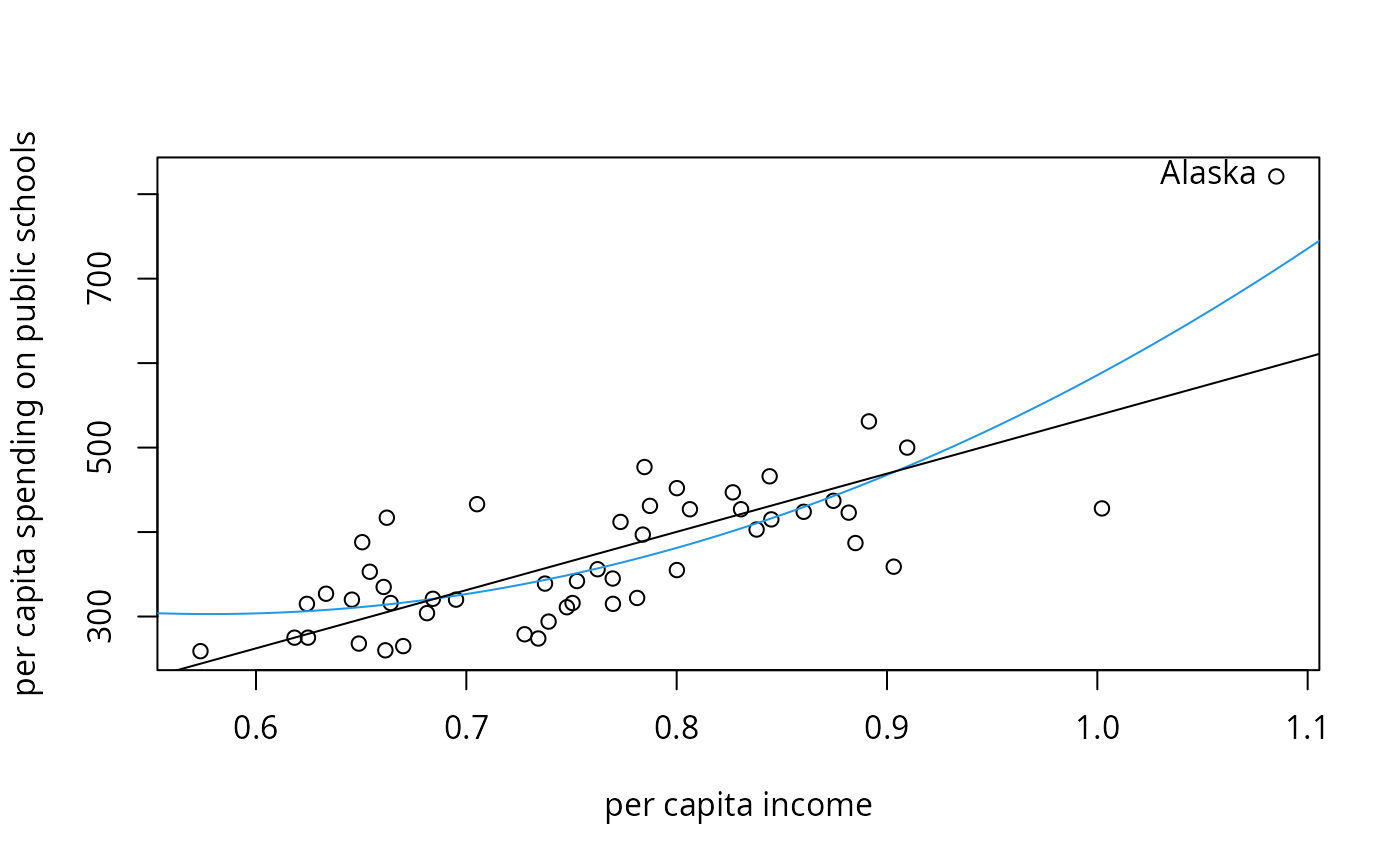
## visualization, p. 230, Figure 1
plot(Expenditure ~ Income, data = ps,
  xlab = "per capita income",
  ylab = "per capita spending on public schools")
inc <- seq(0.5, 1.2, by = 0.001)
lines(inc, predict(fmq, data.frame(Income = inc)), col = 4)
fml <- lm(Expenditure ~ Income, data = ps)
abline(fml)
text(ps[2,2], ps[2,1], rownames(ps)[2], pos = 2)